Two Simple Examples

The first operations that may come to mind using self-similarity involve a fractal as a set of pitch sequences. We will first present two very simple examples which, we think, will make the method more clear. The score for audio example 4 is printed in table 5.2; the values used in this example are similar to the example explained in table 5.1.

Table 5.2: The score for audio example 4.

At the end of the score is the definition for the ``mainseed''; it defines an initial value of ``init'', which is a point, a structure (``twopoint'') and a production object (``snd''). The structure ``twopoint'' is composed of two points ``a1'' and ``a2'', which define an equal binary time segmentation (0.5,0.5) and frequency multipliers of 1 and 2. The option ``lastlevel'' means that we will only use the last level cells of the developed parameters. Both of these points refer to the mainseed; therefore, we have a single level recursive hierarchy. The object ``snd'' defines the sound production values. Since the system has no way of knowing how long the synthesized sound is going to be, we have to specifically define the allocation of the sound buffer, and that is specified by the ``time: 10.0'' entry. The ``srate'' entry defines the sampling rate, and ``file'' specifies the file name to which the produced sound will be written. As discussed before, ``window'' defines an amplitude window whose length is adjusted to the length of the cell; for now we can ignore this entry since we are not applying a window in the process. (Actually, we are applying the window ``nowin'', which is just a constant value of 1.) A sinusoid table is used by default for a table lookup, and the ``stop_rec'' (which stands for ``stop recursion'') specifies a time threshold for the last level of parameter development. We will stop the parameter development process, once we reach a cell whose duration is less than the value of the ``stop_rec''. The point ``init'', which is the initial value of the ``mainseed'', specifies that we are asking for 2 seconds of sounds to be synthesized while the initial values for the development of the frequency and amplitude parameters are 100, and 0.1 respectively. This score will produce a sinusoid whose frequency is ascending fractally. The frequency fluctuation of this example as well as the frequency fluctuation of half of its duration is illustrated in figure 5-1.

Figure 5-1: The frequency fluctuation of the audio example 4 is illustrated. (a) shows the frequency fluctuation in 2 seconds and (b) shows the frequency fluctuation in 1 second. The basic shape of both graphs are similar to each other.

The similarity of the two graphs can be seen as four broken lines ascending in 1 or 2 seconds.

In the next example we will show the use of expressions and make the self-similarity of the frequency fluctuation clearer by a trinary segmentation of time. The score for audio example 5 is printed in table 5.3.

Table 5.3: The score for audio example 5.

The basic shape of the hierarchy of this score is the same as the first example, except that the structure of this example is composed of three points (using the point ``a1'' twice). The time factor is defined as an expression, and the frequency factors used are 1 and 1.5. Expressions have to be quoted with backquotes (`). In expressions there is no assumption about how the higher level values are treated, and any operation has to be explicitly specified. In this case the variable ``time'' in the expression `time / 3` implies that the duration of the cell in the current level is one third of the duration of the higher level cell. If we had simply used a value of 0.333 for the time entry in ``a1'', then we had to use a value of 0.334 for the time entry in ``a2'' to make sure that the duration of all of our cells in every level adds up to be the same. It is legal to use time segmentation factors which do not add up to 1. However, that should be used with the knowledge of how the global time is managed in the system, so that undesired side effects would be avoided. The system parses the recursion tree depth first, and advances the global time anytime it reaches the ``stop_rec'' value in the last level. Therefore, if we used values which did not add up to 1, as we get deeper into the recursion tree the addition of the cell duration becomes smaller, and finally we will create a sound shorter than what we had initially asked for. All of the values of all the higher level factors can be used in an expression. For example `freq + 10` means that the value of the frequency factor in the current level is equal to the value of the frequency factor in higher level plus 10. Factors can be indexed as arrays to access values of factors in the levels not immediately preceding the current level. For example, `freq[1] + 10` means that the value of the frequency in the current level is equal to the value of the frequency factor in two levels above. Notice that `freq + 10` is a shorthand for `freq[0] + 10`. Currently two global variables are recognized: ``rec_level'' is the value of the current recursion level and ``cur_time'' is the value of the currently advanced global time. 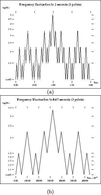Let us get back to our examples. Figure 5-2 illustrates the frequency fluctuation of the audio example 5. In this case the self-similarity of the frequency fluctuation is rather apparent.

Figure 5-2: The frequency fluctuation of the audio example 5 is illustrated. (a) shows the frequency fluctuation in 2 seconds and (b) shows the frequency fluctuation in 0.667 second. The basic shape of both graphs is a triangle.

The next step is to use all the values of the factors in all levels for synthesis. The result will be as if we had synthesized a signal for every level of the parameter development (as described above) and had added all the signals together. The system takes this action by default, unless the ``lastlevel'' option is set. The score for audio example 6 is printed in table 5.4, which is the same as the previous example without the ``lastlevel'' option.

Table 5.4: The score for audio example 6.

Notice that we have used amplitude factors of 0.6, so that the higher frequency partials would have lower amplitude. We have also used a value of 2.08286 for the duration of sound, so that the number of samples can be divided by 3 up to the point that we stop the parameter development. This is an important issue in this example since we are not using any amplitude window for the cells. Had we used a value of 2.0, we would have produced clicks due to the round-off error of calculating the number of samples of the duration of every cell. Finally, we can hear the additive version of our first example as audio example 7, whose score is printed in table 5.5. In this example we have used the ``loop'' option of the sound object and looped the result 3 times.

Table 5.5: The score for audio example 7.